The other day I wrote a piece that used a bit of data to question peoples beliefs (on both sides of the spectrum) about when should English Premier League clubs start to recruit players (Baby England : Scout Onwards).
The piece stimulated a bit of debate on Twitter with two camps of thought clearly emerging; 1) Talent is Talent – Scout them early! 2) What the hell are they doing!
The debate has encouraged me to further the data collection process that was completed for Baby England, in order to create a more worldwide view. The results and discussion on the new data is presented after a brief detour. The debate on twitter touched on a few different areas of research and its worthwhile delving into some of the thinking that is generating this schism of thought:
Camp 1: Talent is Talent – Scout them early!
“Premier League Teams are scouting players early and they are making it to the England Senior Team, so its working… The reason its working is because talented players are talented from an early age its quiet simple. After 16 its only Smalling and Carrick – England are fine without them. Also… just look at Messi when he was 7”
Camp 1 Spokesperson, 2016
Evidence 1:
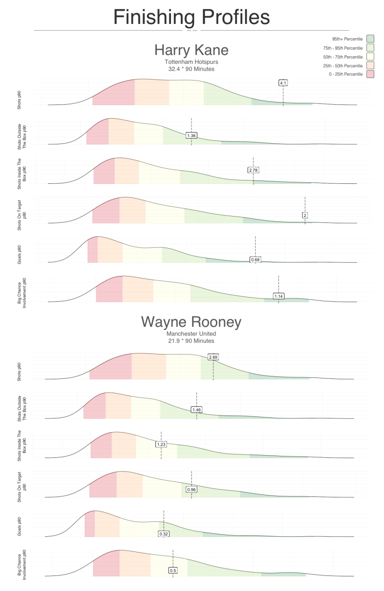
Evidence 2: See 1:14
“Case Closed!”
Camp 1 Spokesperson, 2
Camp 2: What the hell are they doing!
The backbone of Camp 2’s argument is that children develop emotionally, mentally, socially and athletically at very differing rates and recruiting players at a young age will let huge amounts of talent drift away. Essentially, ‘Selection Bias’ – we will use the concept of Relative Age Effect (RAE) to explain that Selection Bias is very evident professional football.
Relative Age Effect
The Relative Age Effect is a phenomenon that suggests that athletes at elite level are more likely to be born in the first 3 months after the eligibility cut-off date for a particular age group in sports. Credit
NB: Eligibility in the UK runs from August – July and elsewhere from January – December
Further Reading :
1. Football talent spotting: Are clubs getting it wrong with kids? – Alistair Magowan (BBC Sport)
2. Relative age effect in european professional football. Analysis by position – J.Salinero et al
3. The ‘Matthew Effect’ – Ross Tucker
Back to ‘Selection Bias’
Simon Gleave was fighting for Camp 2 and stated:
Based on the evidence found within RAE research, it is logical to think that Simon’s point does have a huge impact on the outcomes for the players selected and also for the players deselected. This point is at the core of Ross Tucker’s philosophy on Talent ID and is expressed excellently in this presentation and explanatory article.
New Research : World Edition
The aim is to look at when ‘successful’ players are signed up to academies in more countries that just England to see if there are any global patterns, evidence of best practice and anything to add to the discussions.
Sample Size
- Countries selected: England, France, Netherlands, Belgium, Italy, Spain, Portugal, Germany, Brazil and Argentina
- All players that have played 10 caps or more for the countries selected for the study
Data Integrity Acknowledgements
- Squad lists for the national teams were obtained from Wikipedia – there are a few casualties of this method (David De Gea and more)
- Each player’s youth team history was gleaned from Wikipedia – there will obviously be some mistakes and inaccuracies
- If a player’s youth history was difficult to ascertain or clarify the age on sign-up he was removed
- In some cases I had to decide if a non-top tier club would count as an ‘academy’, I will have made some mistakes in classification.
- I used ‘Peak Career Market Value’ from Transfermarkt as a proxy for quality. Some players are yet to reach their peak value.
Results : Overview 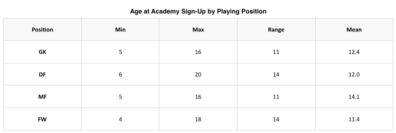
Results: Volume Distribution

Results : Per Country Volume Distribution
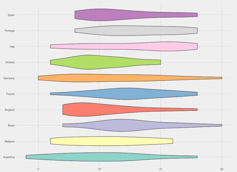
- There is obviously a lot of differences depending on the country with Germany looking like ‘The Sausage of Equality’, England visually differing from others.
- Italy is the only country to have its widest distribution during/post adolescences
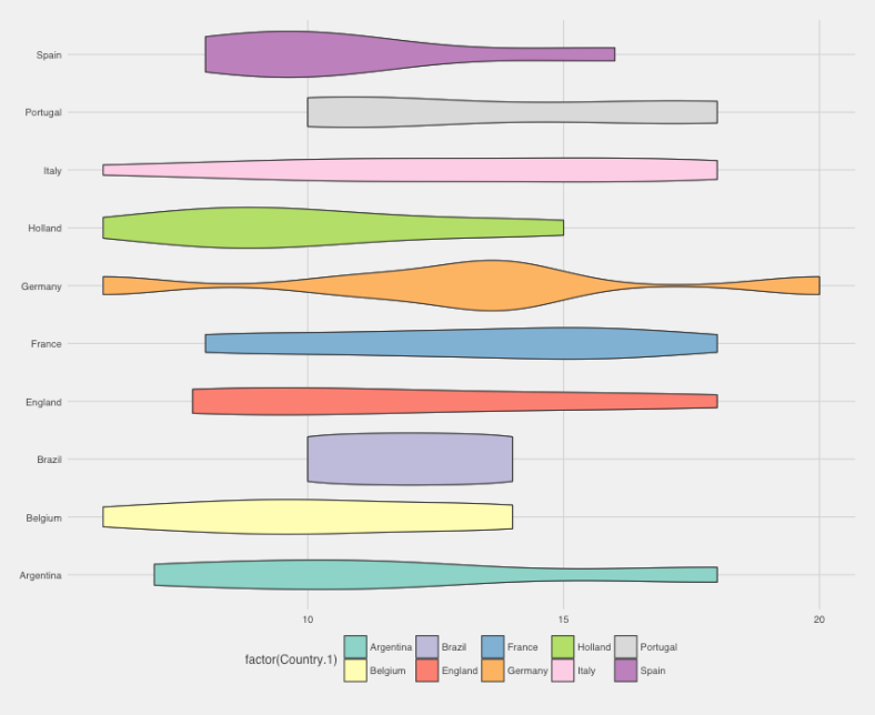
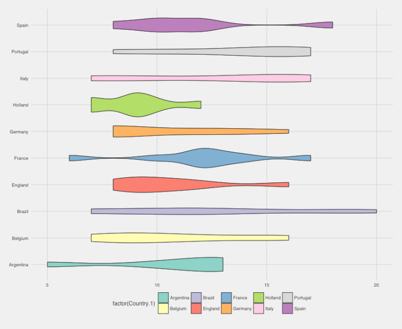
Results : Per Country Volume Distribution – by Position
Goalkeepers:
Defenders:

Midfielders:
Forwards:
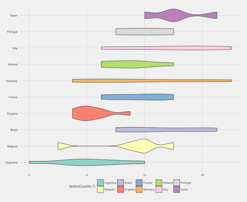
- England’s desire to find their forwards early is amazingly evident, especially when compared to Spain.
- Germany’s ‘Sausage of Equality’ is once again a joy to behold!
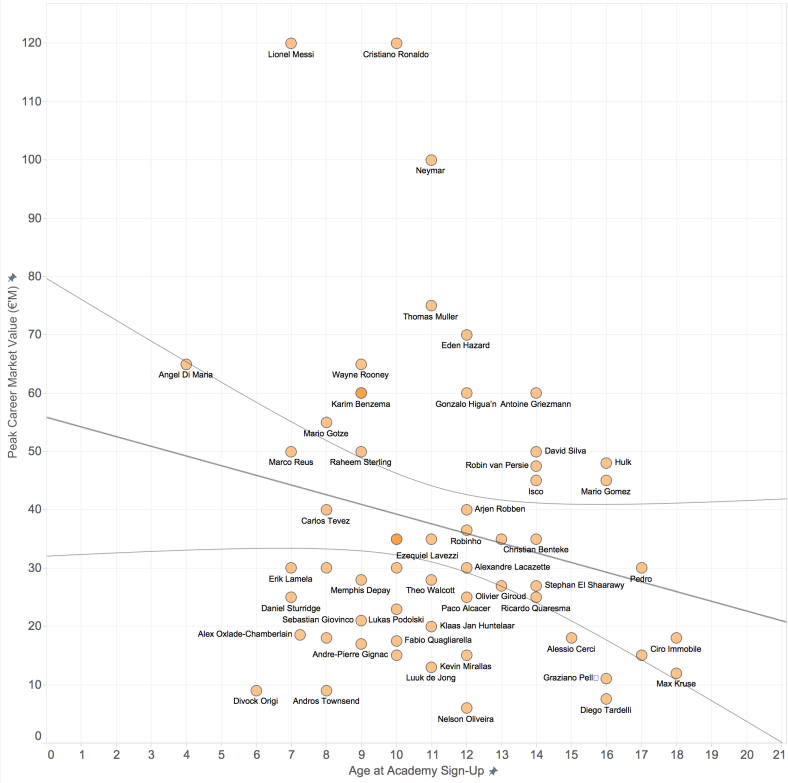
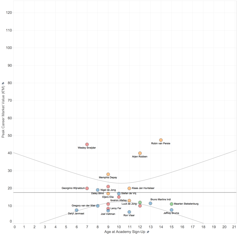
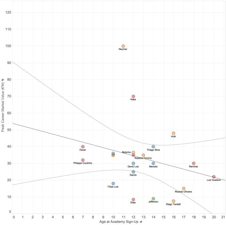
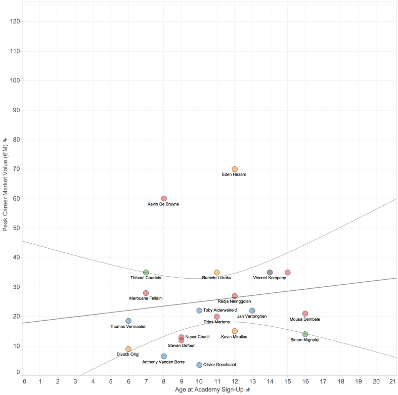
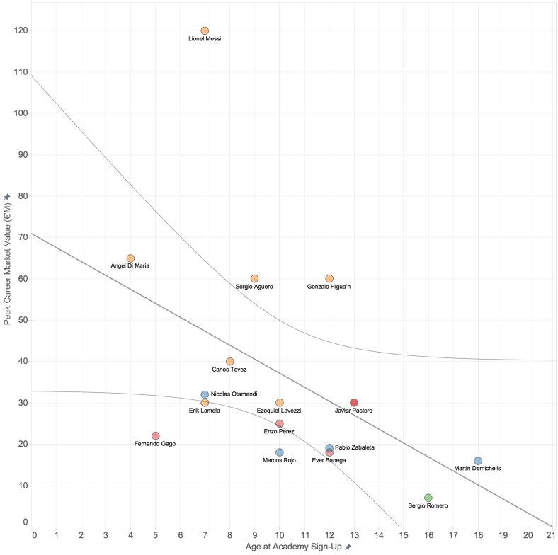
Results: Are the Best Players Found Early?
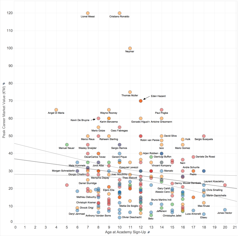
- There is a general linear relationship observed with the tightest confidence brackets at the age of 11.
- There are some big names recruited after 16 – Sergio Busquets!
- Angel Di Maria is the youngest player to be signed up to an academy at aged 4… the transfer fee was 35 footballs.
Results: Are the Best Players Found Early? – by Position
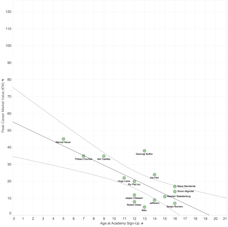
Goalkeepers:
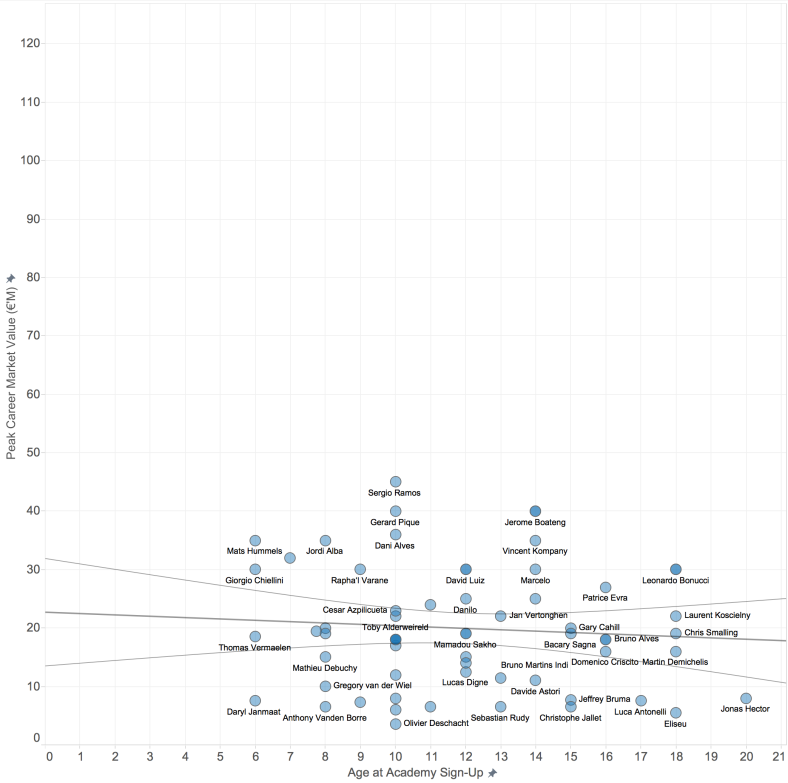
Defenders:
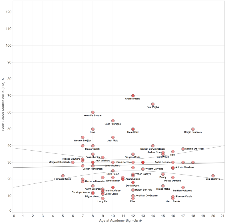
Midfielders:
Forwards:
- Interestingly goalkeepers join forwards as the positions where more value will be found at a young age group
- There is a slight trend towards finding better midfielders later in children’s development
- I would prefer to pick my back 4 from a group that were signed at 10 or below… maybe personal preference.
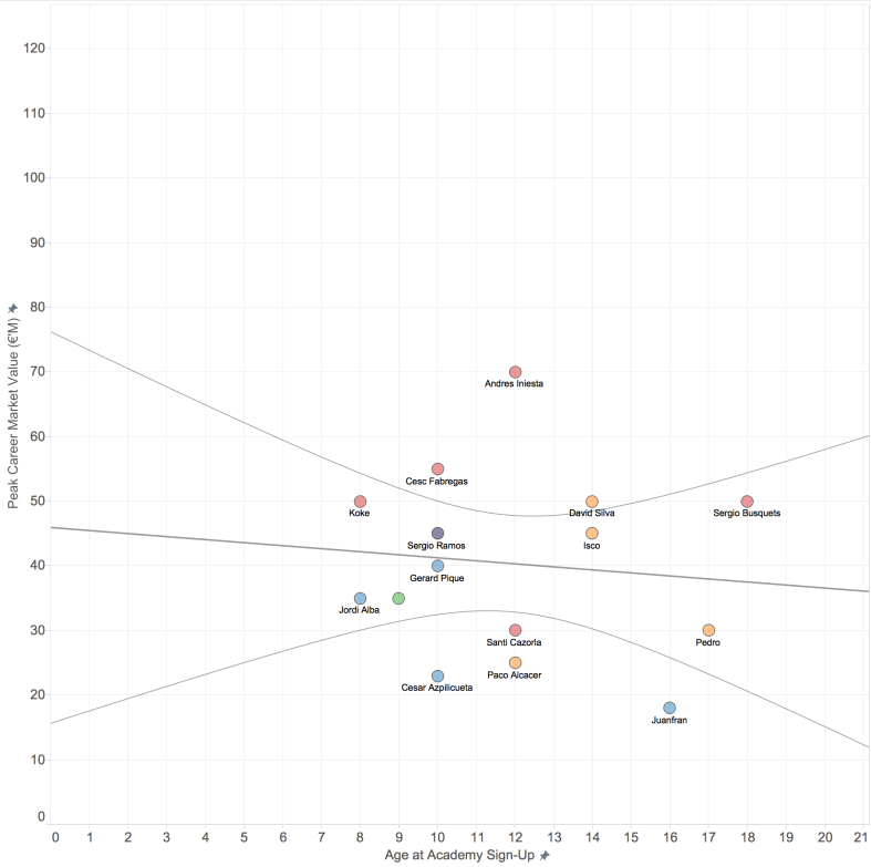
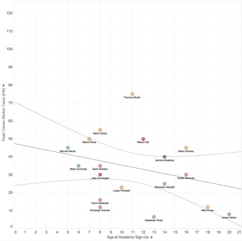
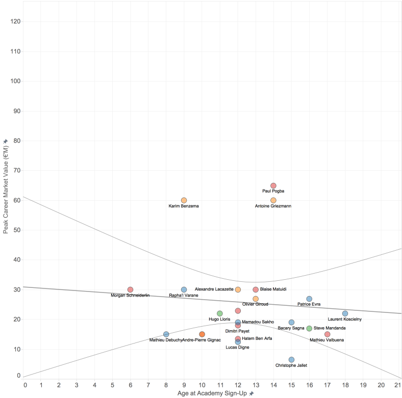
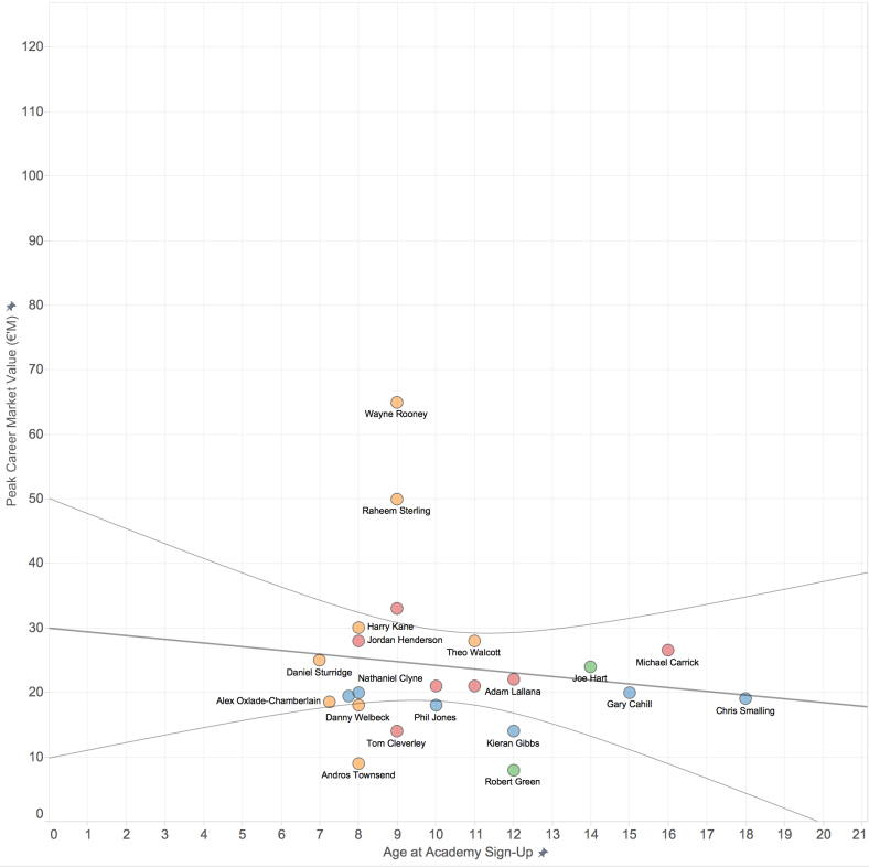
Results: Are the Best Players Found Early? – by Country
Spain:
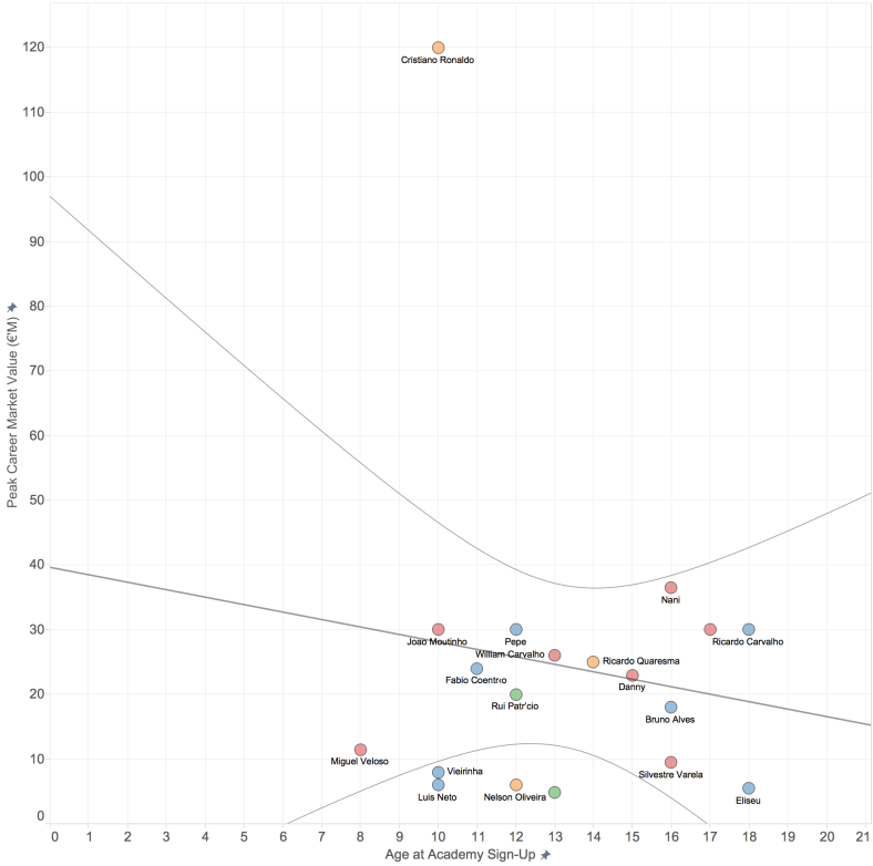
 Portugal:
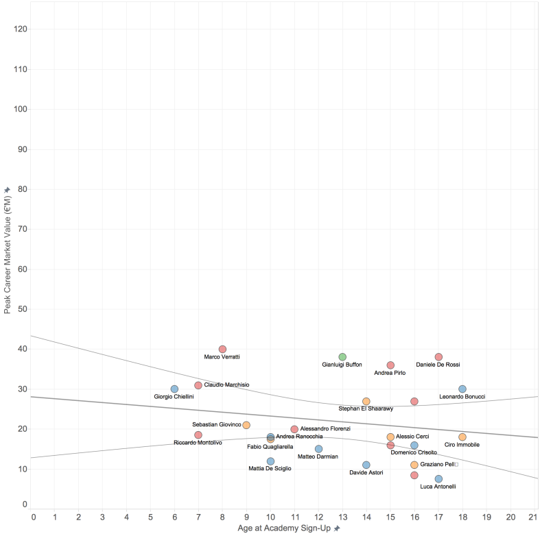
Italy:
Holland:
 Germany:
 France:
England:
Brazil:
 Belgium:
Argentina:
- To be honest, I am not sure what insights to draw from these charts… any suggestions?
- Germany’s plot is interesting as its so wide and open, players of differing values joining at differing times.
- Argentina’s plot potentially shows a football culture / infrastructure where the best young players can gain exposure to scouts… but I am clutching at straws.
Relative Age Effect on Show?
- RAE is very clearly visible and active within this sample size
- Interestingly, the age of academy sign-up of 3rd and 4th quarter players is higher, suggesting that late-developers are spotted but scouts have a tendency to get drawn towards ‘older’ players at the younger ages.
Germany vrs England
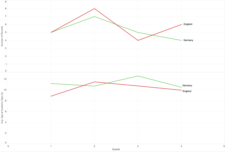
- 1st plot: Interestingly Germany shows a RAE that is closer to the average of the sample size
- 2nd plot: Although the age’s are comparable, this does suggest that Germany are better at identifying/developing ‘late bloomers’
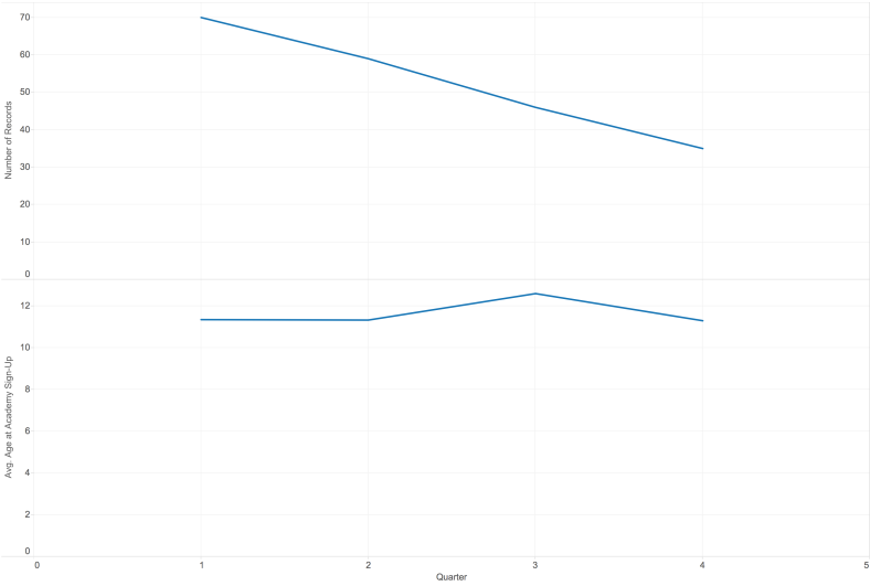
The Race to the Bottom
Ross Tucker writes: (link)
The answer to that question should be clear by now. The major sports teams have engaged in a progressive race to the bottom because of competition between themselves, and also between sports. This latter battle cannot be ignored – Real Madrid can lose out to Barcelona when a potentially great football player chooses the Catalans, or they could lose out to rugby if that player decides to stay in Argentina to play for the Pumas. Similarly, track and field loses to basketball, rowing to rugby, rugby to football, triathlon to swimming, and so on.
And so is created a competitive market where supply is very limited, but demand is enormous. The cost doesn’t appear until much later, however, when the player reaches maturity and the ‘bet’ made by the team has actually come to maturity. That is, Messi was a bargain at 8, he was getting costly by 15, and by 21, priceless.
Therefore, what the major sports have done is assess their desire for efficiency, and given how much money they have, realised that it doesn’t actually matter if they waste $100,000 on 100 players (cost of $10 million), because if the 101st player is Lionel Messi, then they’re way ahead of the game. That’s not to say they don’t care at all – if they could find a Messi once every 50 rather than 100 players, then they save $5 million, but the cost of NOT identifying him is enormous. That’s the opportunity cost I spoke of earlier, and to wealthy sports and teams, this is the driver, not expense.
Can we see this ‘Race to the Bottom’ from the sample size?
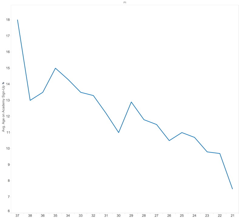
- There is a trend that clearly agrees with Ross Tucker and shows the Race for the Bottom
- However, this may well be down to sample size issues and we have to take the graph with a pinch of salt.
- That being said, the Race for the Bottom is something that most of the readers will agree that exists.
Conclusion:
- Elite talent can be found at a younger age, therefore clubs have to scout at a young age. Significant talent is snapped up by aged 8, therefore due to economic realities clubs will and should scout at these age groups.
- ‘Late-Developers’ or ‘Over-Looked Talent’ is a major market!! To name a few: Sergio Busquets, Daniele De Rossi, Paul Pogba, David Silva and many more. England are very poor in recruiting from and developing the late-developers. However, I feel it’s an easy argument to make against the clubs and the scouts. The majority of the burden should be carried by the English FA for not implementing structures elite development / coaching outside of the club system. Unlike in Germany, where there are expert coaches working with talents that were not selected by the professional clubs, in England those players can languish in their grassroots teams and continue to be coached by parents or volunteers. The DBF have taken the responsibility for the development of the ‘deselected’ and that is why we see Germany’s impressive ‘Sausage of Equality’.
- Camp 2 are definitely the winners! However, they must concede that it is worthwhile aggressively scouting and recruiting the best U8s. Yet this has to be balanced with acknowledgment of the RAE and a contribution to the development of ‘deselected’ talent.
Closing Take Home
I can’t find the tweet now, but Simon Gleave tweeted something along the lines of:
“The academy that takes advantage of the talent left behind from recruiting ‘old’ players will see huge benefits”
Simon – please feel free to correct me on the above…